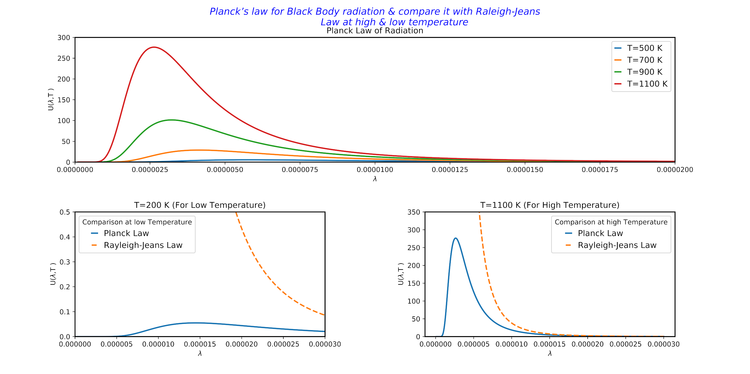
Plot Planck’s law for Black Body radiation and compare it with Raleigh-Jeans Law at high temperature and low temperature using Python :
Planck's Law: Planck's law, also known as Planck's radiation law, is a theoretical formula that describes the spectral density of electromagnetic radiation emitted by a black body in thermal equilibrium at a given temperature. The law states that the energy density per unit wavelength interval of black body radiation is proportional to the fourth power of the temperature and inversely proportional to the fifth power of the wavelength. The law was proposed by Max Planck in 1900 and it played a crucial role in the development of quantum mechanics.
Algoritham :
=>Importing necessary libraries such as numpy for array creation ,matplotlib for plot the graph and scipy for get constant value .
=>Now define an array for wavelength range such as L=np.arange .
=>Now define function planck_lamda for Planck law of black body radiation .
=>Write the equation of Rayleigh-Jeans law for high and low temperature .
=>Using 'plot' command for plot the graph .
=>Using 'xlim' and 'ylim' command for limiting the graph .
=>Using 'legend' command for comment on graph .
=>Using 'xlabel' and 'ylabel' command for level the graph and for graph title using 'plt.title' command .
=>Finally , using 'plt.show()' command for show the graph on the screen .
Source code :
  """ -Statistical Mechanics LAB
Q.Plot Planck’s law for Black Body radiation and compare it with Raleigh-Jeans Law at high
  temperature and low temperature.
 """
import numpy as np
from scipy.constants import h, c, k, pi
import matplotlib.pyplot as plt
newparams = {'axes.labelsize': 10, 'axes.linewidth': 1.5, 'savefig.dpi':
      1000,
     'lines.linewidth': 2, 'figure.figsize': (18, 12),
     'legend.frameon': True,
      'legend.handlelength': 0.7}

plt.rcParams.update(newparams)

L0 = np.arange(0.1,30,0.005) #Wavelength in micro m
L = L0*1e-6 #wavelength in m


def planck_lamda(L,T):
     a = (8 * pi * h * c) / L **5
     b = (h * c)/ (L * k * T)
     c1 = np.exp(b) - 1
     d = a / c1
     return d
plt.suptitle("""Planck’s law for Black Body radiation & compare it with Raleigh-Jeans
             Law at high & low temperature""",
          size = 14,color='b',fontstyle ="italic")

R_Ht = (8* pi *k *1100)/L**4 #Rayleigh's law at High temperature
R_Lt = (8*pi*k*200)/L**4 #Rayleigh's law at Low temperature

T500 = planck_lamda(L , 500)
T700 = planck_lamda(L , 700)
T900 = planck_lamda(L , 900)
T1100 = planck_lamda(L , 1100)


""" ##### Sub plot creation ##### """
plt.subplot(2,2,(1,2))
plt.plot(L, T500,label='T=500 K')
plt.plot(L, T700 ,label='T=700 K')
plt.plot(L, T900 ,label='T=900 K')
plt.plot(L, T1100 ,label='T=1100 K')
plt.legend(loc="best" ,prop={'size':12})
plt.xlabel(r"$\lambda$ ")
plt.ylabel(r"U($\lambda $,T )")
plt.title("Planck Law of Radiation")
plt.ylim(0,300)
plt.xlim(0,0.00002)


plt.subplot(2,2,3)
plt.plot(L, (planck_lamda(L,200)),label='Planck Law')
plt.plot(L, R_Lt , "--" , label="Rayleigh-Jeans Law")
plt.legend(title="Comparison at low Temperature",loc="best" ,prop={'size':12})
plt.xlabel(r"$\lambda$ ")
plt.ylabel(r"U($\lambda $,T )")
plt.title("T=200 K (For Low Temperature)")
plt.ylim(0,0.5)
plt.xlim(0,0.00003)


plt.subplot(2,2,4)
plt.plot(L, T1100 ,label='Planck Law')
plt.plot(L, R_Ht , "--" , label="Rayleigh-Jeans Law")
plt.legend(title="Comparison at high Temperature",loc="best" ,prop={'size':12})
plt.xlabel(r"$\lambda$ ")
plt.ylabel(r"U($\lambda $,T )")
plt.title("T=1100 K (For High Temperature)")
plt.ylim(0,350)


"""###### Sub plot Adjusting ######"""
plt.subplots_adjust(left=0.1,
                    bottom=0.1,
                    right=0.9,
                    top=0.9,
                    wspace=0.4,
                    hspace=0.4)


plt.show()
Result :
 |
| Plot of Planck's law of black body radiation |
| Learn Basic of Python |
| C programming Tutorial |
| Creat Simple calculator using C++ programming |
| Find factorial value of any number using java Programming language |